How to Conduct a Repeated Measures MANCOVA in SPSS
In today's blog entry, I will walk through the basics of conducting a repeated-measures MANCOVA in SPSS. I will focus on the most basic steps of conducting this analysis (I will not address some complex side issues, such as assumptions, power…etc). Full disclosure: the example data used is from the SPSS sample/help files, and it can be downloaded below.
RIGHT-CLICK HERE AND "SAVE AS FILE" FOR SAMPLE DATA
Let's get started:
Repeated-Measures MANCOVA is used to examine how a dependent variable (DV) varies over time, using multiple measurements of that variable, with each measurement separated by a given period of time. In addition to determining whether the DV itself varies, a MANCOVA can also determine wether other variables are predictive of variability in the DV over time. If that wasn't crystal clear, don't worry, just keep reading.
Repeated-Measures MANCOVA Example:
In our example, your local stats store Stats "R" Us launched a marketing campaign, with three different strategies (variable name:
promo; value labels: Strategy A, Strategy B, Strategy C). Stats "R" Us launched campaigns in markets of three different sizes (variable name: mktsize; value labels: Small, Medium, and Large), and measured the sales in each store every three months over the course of one year (4 time points; variable names: sales.1, sales.2, sales.3, and sales.4; see data below).

NOTE: Sales are scaled in "thousands" (e.g. 70.63 is actually $70,630). Also, your data should be in person-level (a.k.a. "wide") format (as opposed to person-period, a.k.a. "long", format), meaning each row of data is a single case (store, in our example). If it were in person-period (long) format, each case (store) would have the number of rows equal to the number of repeated measures (four, in our example), because the repeated measures (sales.1, sales.2, sales.3, and sales.4) would be stacked to form a single variable (Sales). Here is a useful resource for converting data between the two forms: CLICK HERE FOR INFO ABOUT CONVERTING DATA FORMS.
To begin your analysis using the SPSS drop-down menus, click on: Analyze > General Linear Model > Repeated Measures... (1, below)

In the Repeated Measures Define Factors dialogue window, do the following:
- Replace the default Within-Subject Factor Name, which is factor1, with your own name for the concept of time. I've chosen to use the name Time (1, below).
- Type the number of times your DV was measured (how many DV variables you have) in the Number of Levels box (2, below) and click the "Add" button.
- Choose a name for your DV (the variable that is measured repeatedly), and type it in the Measure Name box. I chose the name Sales (3, below).
- Click the "Add" button again (4, below).
- Click the "Define" button (5, below).


In the Repeated Measures dialogue window that appears next, move the four sales variables (1, below) to the Within-Subjects Variables (Time) box (2, below).
NOTE: Be sure that they stay in the same order (Sales.1, Sales.2, Sales.3, and Sales.4).


Next, move both promo and mktsize to the Between-Subjects Factor(s): box (1, below).
NOTE: Both promo and mktsize were placed into the Between-Subjects Factor(s) box because they are categorical variables (discrete variables). Continuous variables (scale variables) would go into the Covariates box (2, below).

Next, click on the "Model" button (3, above).
In the Repeated Measures: Model dialogue window (1, below), you can specify your model. In other words, you can choose which variables have "main effects" on the DV (individual predictors), and which variables might interact with each other to predict the DV. The default option is the Full factorial (2, below), which will examine every variable's main effect, as well as every possible interaction among all variables.

We'll stick with Full factorial for today. However, if you wanted build your own model, you can choose Custom (1, below), and then use the Build Term(s) tool (2, below) to specify what kind of effects/interactions you want. Again, in this example, we'll stick with Full factorial (2, above). To exit this dialogue window, click the "Continue" button.

Next, you'll need to click on the "Contrasts" button (1, below). In the Repeated Measures: Contrasts dialogue window that appears, you can change each factor variable's type of contrast. I recommend leaving the Time variable with its default contrast "Polynomial" (2, below), and changing both promo and mktsize to "Simple" and "First". To change each, you must select "Simple" from the list, click on "First", and then click on the "Change" button (3, below).

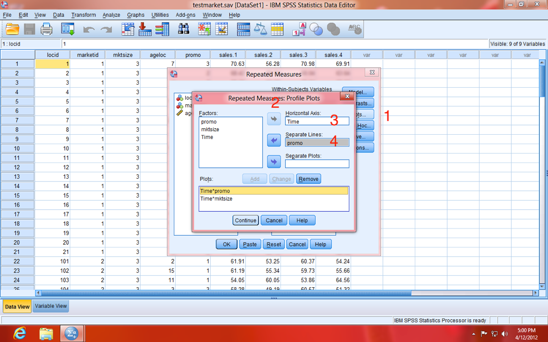
Next, click on the "Plots" button (1, below). In the Repeated Measures: Profile Plots dialogue window that appears (2, below), you can choose what graphs you'd like to see. In repeated measures models, I like to produce plots with Time on the Horizontal Axis (x-axis; 3, below) and my factor variables as Separate Lines (4, below).
NOTE: The reason you don't see anywhere to specify the vertical axis (y-axis), is that the DV (i.e. Sales) is assumed to be on the y-axis in this dialogue window.
As you can see, in our example I've made a Time-by-Factor plot for each of the factors in our model (promo and mktsize).
If you'd like to get Post Hoc comparisons of the DV (comparing between each of the factor levels, respectively), click on the "Post Hoc" button. Once in the dialogue window:
- Move the factors from the Factor(s) box (1, below) to the Post Hoc Tests box (2, below).
- Choose the type of Post Hoc test to use, and place a check-mark in its respective box (you can choose more than one). The most commonly used is Tukey's, which I've chosen below (3, below).
- Click the "Continue" button.

I also recommend clicking on the "Save" button (1, below), and choosing Predicted Values:Unstandardized (2, below) and Residuals: Unstandardized (3, below) in the Repeated Measures: Save dialogue window.
NOTE: By checking these two boxes, your analysis will now produce two new variables in your dataset, called PRED_1 (Predicted) and RES_1 (Residual), which can be used to produce graphs after analysis (if you choose). We will not cover this in this tutorial.

Back at the main Repeated Measures dialogue, you can either click "OK" (1, below), to execute the analysis, or you can click "Paste" (2, below), to paste the analysis commands into a syntax window. I recommend choose the "Paste" option, as that will allow you to more easily re-create the analysis later.

Below is the syntax window, with the various commands of the analysis, which you specified while going through the dialogue windows. Over time, you may learn to use syntax exclusively, bypassing the need to use the dialogue windows. Learning syntax can dramatically improve your efficiency, especially when you need to create a lot of different types and/or iterations of analyses.

To execute the commands in the syntax, simply highlight all the text you want to run, and push the green play button (1, above). Alternatively, you can use the menus: Run > Selection.
Interpreting Output/Results
There is a lot to digest in the output file that results from an analysis, so we'll stick to the basics. Below is the Descriptive Statistics table, which simply shows the Mean (1, below), Standard Deviation (Std. Deviation; 2, below), and sample size (N; 3, below) for each DV, broken-down by all subgroups of your factors (promo and mktsize).

The next table we'll examine is the Mauchly's Test of Sphericity. This test essentially determines whether the variance of the difference between each pair of repeated measure (of your DV) is approximately equal. This is a bit of an over-simplification, but it'll work here. For our purposes, we just need to be concerned with whether it is significant or not (1, below). If it is NOT significant (i.e. Sig. is greater than .05), then sphericity can be assumed (more on that soon). If it IS significant (i.e. Sig. is less than .05), then sphericity can not be assumed (more about why we care, in a moment).
NOTE: I know I said earlier that we wouldn't deal with assumptions today, but this is an exception, because it directly determines how we interpret the next table...
In our example, we CAN NOT assume sphericity (p=.003).

The reason we want to note whether sphericity can be assumed, is that it directly determines how we interpret our next table, the Tests of Within-Subjects Effects table (1, below). For each effect in our model, there are four estimates present (2, below). If sphericity CAN be assumed, then we can reference the first estimate, aptly labeled Sphericity Assumed. If sphericity CAN NOT be assumed, then we'll want to reference one of the other three (the differences between them is somewhat esoteric, but I typically choose Greenhouse-Geisser). In either case, we reference the Sig. column (3, below) to determine whether our effects are significant.
In our example, we see that we had no significant effects. Since we could NOT assume sphericity, the Greenhouse-Geisser test tells us that Time was not a significant predictor of Sales (i.e. there was no overall positive or negative trend in Sales in the company as a whole), F(2.743, 340.097)=.743, p=.516, ηp2=.006.
We also see that neither promo F(5.485, 340.097)=.660, p=.668, ηp2=.011, nor mktsize F(5.485, 340.097)=1.048, p=.391, ηp2=.017 interacted with Time to predict trends in Sales. Additionally, there was also no significant three-way interaction between Time, promo, and mktsize F(10.971, 340.097)=.940, p=.502, ηp2=.029. Take note of how I report those statistics , as it is necessary for APA format.

The next table was produced because we chose the "Polynomial" contrast for Time earlier. It is very useful in case non-linear relationships exist in your data. More specifically, it determines whether there is a Linear or a non-linear relationship exists, such as Quadratic or Cubic (1, below). The more nuanced differences between these effects is beyond the scope of this blog, but Notre Dame's Dr. Richard Williams explains it well in his page on Non-linear Relationships.

The Tests of Between-Subjects Effects table (below) shows whether the factors were associated with differences in Sales (overall, as opposed to whether there were differences in trends).
Results indicate that both promo F(2, 124)=12.837, p<.001, ηp2=.172 and mktsize F(2, 124)=15.085, p<.001, ηp2=.196 were predictive of differences in Sales (overall), while the interaction between the two was not significant F(4, 124)=.186, p=.945, ηp2=.006. These results may seem a bit confusing, because they are in direct contrast to the within-subject effects reported earlier, but it will become more clear when we examine the plots of the effects next.

The plot below shows the mean Sales at each of the four data collections, for stores using each of the three promotional Strategies (three lines). The graph demonstrates that there are distinctions between sales numbers of the three strategy groups, as (Strategy A was highest at every time point and Strategy B was lowest at every time point). However, since the trend for each group (if you were to impose a trendline across the four points for each group) is not dramatically different (and because the interaction term was not significant), we can't clearly say that one promotional strategy is superior to the others.
Since, the differences between groups at time pionts 2, 3, and 4 are largely reflective of the differencs that existed at baseline (time 1), it seems that differences that exist between groups are more likely attributed to differences in the composition of the groups, rather than differences in the promotional strategy. The graph for mktsize can be interpreted in the same way as promo.

This graph further shows how it is better to examine within subject differences when analyzing change over time, as plotting those effects makes the lack of differences in trend between promo groups more clear. Thanks for reading and please leave comments and/or questions!